In this post, I’m going to describe a method I’ve been working on for performing probabilistic tractography in a single subject using automatically generated cortical labels from Freesurfer. This isn’t new or groundbreaking, however the description of such methods as found in a paper is generally a lossy transmission of the actual code used to generate this kind of analysis.

Scientific replicability & reproducibility require a working implemention and I’ve not seen such a description of this kind of analysis & processing in the internet, hence this article. I hope this is helpful to the community. It’s also taken a lot of time for me to get here so hopefully you won’t have to make the same mistakes I have (but mistakes are good so hopefully you make your own :)

I’m making certain assumptions & decisions in this analysis. If you don’t agree with them, that’s alright, you’re not going to hurt my feelings. It doesn’t make this any more or less correct. This is an immature technique and I don’t think there are hard & fast rules the field has yet approved for cortical tractography. But if you think something is really wrong, I’d love to get your opinion, discuss it and potentially update this post.

The goal of this analysis is to get a measure of structural connectivity between all cortical “regions” of the brain. There are an infinite amount of ways to divy up a brain into regions of interest. Here, I’m choosing to use the 2009 labels produced by Freesurfer Destrieux atlas. Using FSL’s probtrackx2 tool, we’ll use DTI data to perform “in-silico tractography” (hand-waving) from each region and measure to what degree each region “connects” to every other region. There are a lot of caveats in the above paragraph & a lot of underlying assumptions I’m making up-to-and-including:

• Freesurfer generates accurate & reliable cortical labels from a clean T1 image.
• Diffusion MRI captures the relative motion of water molecules in tissue.
• Water most likely moves parallel to axons which carry action potentials from the neuron to their target.
• Action potentials are the primary means neurons use to communicate with one another.
• During development, the brain organizes itself in such a way that groups of neurons that communicate often with other groups will develop large axonal bundles between one another.
• These bundles restrict the diffusion of water in a way that is detectable during a diffusion MR sequence.
• Using the diffusion information, we can build probability density functions at every voxel to describe our best guess at which way water flows at that particular voxel. These PDFs also help us characterize the uncertainty inherent in the measurement.
• Using these PDFs, we can step through the diffusion image, generating the most likely path water would flow beginning at some point A. We call this a tract, streamline or sample.
• Generating lots of these potential tracts, we can make statistically sound inferences about whether we actually trust that the generated tracts represent the actual underlying anatomy. The actual anatoamy is otherwise difficult to attain from our subjects, hence why we’re imaging them.
• Pulling this large amount of data together, we can generate a NxN connectivity matrix and plot the relative connectivity between all regions.

If I haven’t offended you with any of these statements, let’s get on with it.

Prerequisites

Data

This analysis requires the following MR data:

1. A Freesurfer-able T1 image. This should cover the entire brain at high-resolution (~1mm³ voxels). For this article, I’m going to call this file T1.nii.gz.
2. A DTI sequence with at least 30 directions, though depending on your SnR fewer directions can be acceptable in certain cases. The standard sequence I use is 60 directions. I’m going to refer to this file as dti.nii.gz.
3. The b-values & b-vectors for the gradients. These files should be generated in the process from converting your raw images (probably in DICOM format) to the standard research format (NIFTI). These are simple text files that I’ll refer to as bvals and bvecs.

We’re going to call this subject janedoe.

$ ls ./
T1.nii.gz      dti.nii.gz         bvecs
bvals

Software

I’ll be using Freesurfer & FSL for this analysis, both of which are freely available. In particular, I use Freesurfer 5.1 & FSL 5.0.6 though I’m fairly certain this will work in the newest version of Freesurfer, 5.3.

Structural processing

The T1 image needs to be processed through Freesurfer’s standard recon-all pipeline. There are many resources for how to do this online, namely the Freesurfer wiki. I run the pipeline this way:

$ recon-all -s janedoe -i T1.nii.gz
$ recon-all -s janedoe -all \
    -qcache \
    -measure thickness \
    -measure curv \
    -measure sulc \
    -measure area \
    -measure jacobian_white
$ mri_annotation2label --subject janedoe \
    --hemi lh \
    --annotation $SUBJECTS_DIR/janedoe/label/lh.aparc.a2009s.annot \
    --outdir $SUBJECTS_DIR/janedoe/label \
    --surface white
$ mri_annotation2label --subject janedoe \
    --hemi rh \
    --annotation $SUBJECTS_DIR/janedoe/label/rh.aparc.a2009s.annot \
    --outdir $SUBJECTS_DIR/janedoe/label \
    --surface white

The first recon-all imports the data and creates the standard folder layout in $SUBJECTS_DIR/janedoe. The second call executes all three steps of the Freesurfer pipeline (note the -all flag). The two mri_annotation2label commands convert the Destrieux cortical annotation to individual labels across the two hemispheres. These labels are written into the label/ directory for the subject. Labels are simple text files that map Freesufer vertices to particular cortical regions.

This process usually takes between 20-40 hours depending on the quality of data. Grab a cup of coffee or a nap.

After this completes, we need to do quality assurance. I’m sure there are more rigorous examples out there but this is what I do. For janedoe, I generate the following tcl scripts:

$ cat janedoe.tkmedit.tcl
for { set i 5 } { $i < 256 } { incr i 10 } {
SetSlice $i
RedrawScreen
SaveTIFF janedoe_screenshots/tkmedit-$i.tiff
}
exit
$ cat janedoe.tksurfer.lh.tcl
make_lateral_view;
redraw;
save_tiff janedoe_screenshots/rh-lateral.tiff;
rotate_brain_y 180;
redraw;
save_tiff janedoe_screenshots/rh-medial.tiff;
labl_import_annotation aparc.a2009s.annot;
redraw;
make_lateral_view;
redraw;
save_tiff janedoe_screenshots/rh-annot-lateral.tiff;
rotate_brain_y 180;
redraw;
save_tiff janedoe_screenshots/rh-annot-medial.tiff;
exit;
$ cat janedoe.tksurfer.rh.tcl
make_lateral_view;
redraw;
save_tiff janedoe_screenshots/rh-lateral.tiff;
rotate_brain_y 180;
redraw;
save_tiff janedoe_screenshots/rh-medial.tiff;
labl_import_annotation aparc.a2009s.annot;
redraw;
make_lateral_view;
redraw;
save_tiff janedoe_screenshots/rh-annot-lateral.tiff;
rotate_brain_y 180;
redraw;
save_tiff janedoe_screenshots/rh-annot-medial.tiff;
exit;

Given these files, I run the following commands:

$ mkdir -p janedoe_screenshots
$ tkmedit janedoe brain.finalsurfs.mgz -aseg -surfs -tcl ./janedoe.tkmedit.tcl
$ tksurfer janedoe lh inflated -gray -tcl ./janedoe.tksurfer.lh.tcl
$ tksurfer janedoe rh inflated -gray -tcl ./janedoe.tksurfer.rh.tcl

We make a folder and then run the tcl scripts in tkmedit and tksurfer. The tkmedit script loops through slices in brain.finalsurfs.mgz (colored by the automatic segmentation with the surfaces overlayed), taking a screenshot every centimeter. The tksurfer scripts make screenshots of the lateral & medial views with and without the Destrieux labels.

At this point we’ve got about 35 pictures to look at and check that segmentation & labeling proceeded normally. In the volume data we’re looking for the colors (the volumetric segmentations) to look accurate and no coloring what is obviously not brain. You also want to ensure the surfaces track well with the image.

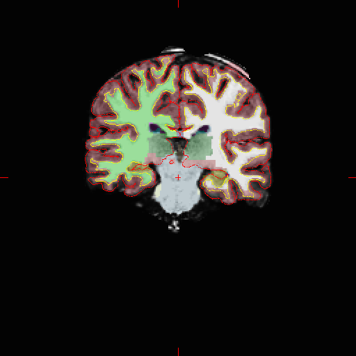
Note that some skull has been left in the what-should-be skull-stripped image and that it’s been labeled as cortex. This is not good but bad results are more enlightening than good ones :)

On the surface images you’re looking for sharp points in the inflated surfaces–these are bad and are most likely to happen on the medial surface (where it’s not quite as important) or in the temporal pole (which is bad if you’re interested in language). With the labels overlayed, one of these screenshots looks like this:

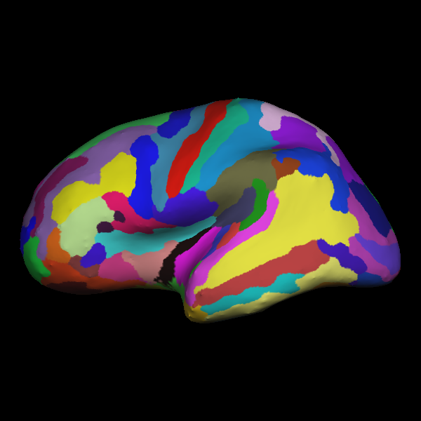
Becuase Freesurfer makes 3D meshes of the white-matter and pial surfaces, we can do fancy things like inflate the brain by pushing out on those meshes. The picture above is the “inflated” view. Each color represents a different labeled region of cortex. Note the spikes in the temporal pole (lowest portion of this view). This is not ideal.

Freesurfer produces a lot of other data . Given the measure flags I passed above to recon-all, more than 2650 data points can be extracted from files in the $SUBJECTS_DIR/janedoe/stats/ folder. If you’re interested in that sort of thing, you might take a look at code I wrote to do just that.

Let’s assume Jane was a great participant and her T1 was very clean. Freesurfer is quite robust and most likely performed good segmentation & labels. On to the diffusion images.

Diffusion Processing

From our DTI data, we need to produce the following information:

1. The mask of the non-diffusion-weighted image.
2. A Fractional Anisotropy (FA) image for registration to the T1.
3. The motion-corrected DTI sequence.
4. PDFs characterizing the underlying diffusion process.

Non-diffusion-weighted mask

For probabalistic tractography, we need to generate a mask within which we constrain tractography. Assuming the first volume of the DTI sequence is the non-diffusion weighted image, we can use bet2 to do this.

$ fslroi dti nodif 0 1
$ bet2 nodif nodif_brain -m -f .25

fslroi extracts the first time volume from the dti sequence and saves it as nodif.nii.gz. Note with FSL commands you do not need to add file extensions. We then use bet2 with a fractional intensity threshold of 0.25. This is generally a robust threshold to remove unwanted tissue from a non-diffusion weighted image. The -m option creates a binary nodif_brain_mask image.

Correcting for Motion

Because we’re collecting many volumes of diffusion-weighted data from our subject, there’s a very high percentage of some motion between volumes. Also because of how the gradient magnets are used to apply a direction of diffusion and then read out the image, lingering currents in the amplifiers can add artifacts to the data. FSL’s eddy_correct tool attempts to fix both issues.

$ eddy_correct dti dti_ecc 0
$ fdt_rotate_bvecs bvecs rot_bvecs dti_ecc.ecclog
$ mv bvecs old_bvecs && mv rot_bvecs bvecs

eddy_correct takes the raw filename, the output filename and which volume to register all of the gradients to (which is typically the non-diffusion-weighted image). This takes a few seconds per volume, so probably around a minute for full data set.

fdt_rotate_bvecs takes the logfile of eddy_correct and applies the proper rotation to the gradient directions. Because we’ve registered every diffusion volume to the first, the original gradients are not accurate anymore. fdt_rotate_bvecs fixes this issue. Then we just rename the new gradient vectors to bvecs without overwriting the old ones.

Generating the FA image

There are much better ways to create an FA image than this method, but as you’ll see below, we’re only using the FA image for registration purposes. I would probably not use this image in a whole-brain FA analysis. For something like that, you might consider using Camino.

$ dtifit -k dti_ecc \
    -o ./dtifit \
    -m nodif_brain_mask \
    -r bvecs \
    -b bvals \

We’re interested in dtifit_FA.nii.gz. dtifit doesn’t implement the most state-of-the-art model of diffusion, but for our purposes its fast and good enough.

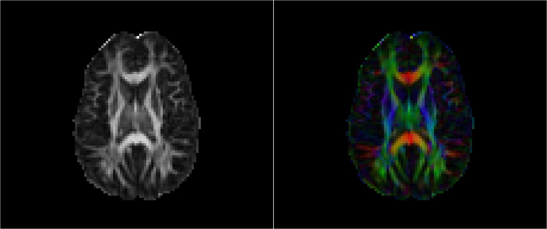
These screenshots were taken with fslview_bin. On the left is the fractional anisotropy (FA) image. In FA images, values varies between 0 & 1 where 0 represents purely isotropic water diffusion. Picture how a golf ball might bounce around inside a basketball–it could go anywhere. Where the FA image is brightest (towards 1), there is one specific direction that water is likely to diffuse (like rolling a golf ball down a paper-towel rod, there isn’t much place else for it to go). FA is typically highest in large fiber bundles such as the corpus callosum (the axonal bundles connecting the two hemispheres). The right image is color-coded by diffusion direction. Green is Anterior-Posterior, Red is Left-Right & Blue is Inferior-Superior (head-foot). The color intensity in this image is modulated by the FA value.

Its very important to look at these images for quality assurance. In the right image, we want to make sure our gradient table is correct and that we haven’t flipped two dimensions. If this were the case, the image would look the same but colors would be switched. In the pure FA image, we’re looking for smearing and other ugly artifacts which typically denote large amounts of motion.

Generating PDFs

At this point we have a motion- & artifact-corrected image (dti_ecc.nii.gz), the corrected gradient table (bvecs), the gradient values (bvals), and a mask of the non-diffusion-weighted image (nodif_brain_mask.nii.gz). If we were smart, we’d use bedpostx out of the box to generate PDFs of the diffusion direction and get on with tractography. Unfortunately, bedpostx takes about 20 minutes per slice and typical datasets contain between 40 and 50 slices so this process takes about 15 hours of compute time. Fortunately, it’s an extremely parallelizable task. So the following script exactly mimics FSL 5’s bedpostx but can run with a linear speedup based on the amount of processors on your machine.

$ cat ./bedpostx.sh

datadir=./

# Estimation parameters
nfibres=2
fudge=1
burnin=1000
njumps=1250
sampleevery=25


mkdir -p bedpostx
mkdir -p bedpostx/diff_slices
mkdir -p bedpostx/logs
mkdir -p bedpostx/logs/pid_${$}
mkdir -p bedpostx/xfms

echo "bedpostx_preproc begin `date`"
bedpostx_preproc.sh ${datadir} 0
echo "bedpostx_preproc end `date`"
echo

nslices=`${FSLDIR}/bin/fslval ./dti_ecc dim3`
[ -f bedpostx/commands.txt ] && rm bedpostx/commands.txt

slice=0
while [ $slice -lt $nslices ]
do
    slicezp=`$FSLDIR/bin/zeropad $slice 4`
    if [ -f bedpostx/diff_slices/data_slice_$slicezp/dyads2.nii.gz ];then
        echo "slice $slice has already been processed"
    else
        echo "${FSLDIR}/bin/bedpostx_single_slice.sh $datadir $slice --nfibres=$nfibres --fudge=$fudge --burnin=$burnin --njumps=$njumps --sampleevery=$sampleevery --model=1">> bedpostx/commands.txt
    fi
    slice=$(($slice + 1))
done

# parallel processing
echo "parallel processing begin `date`"
run_parallel.py bedpostx/commands.txt --ncpu 12
echo "parallel processing end `date`"
echo

# Clean things up
echo "bedpostx_postproc begin `date`"
bedpostx_postproc.sh ${datadir}
echo "bedpostx_postproc end `date`"
echo

$ cat run_parallel.py

#!/usr/bin/env python
# -*- coding: utf-8 -*-

""" run_parallel.py

Simple script to run a list of shell commands in parallel.

"""

import sys
import multiprocessing as mp


def create_parser():
    from argparse import ArgumentParser, FileType
    ap = ArgumentParser()
    ap.add_argument('infile', type=FileType('r'),
        help="file with shell commands to execute")
    ap.add_argument('-n', '--ncpu', type=int, default=0,
        help="Number of CPUs to use (default: %(default)s: all CPUs)")
    return ap


def cpus_to_use(ncpu):
    return ncpu if ncpu else mp.cpu_count()


if __name__ == '__main__':
    from subprocess import call

    ap = create_parser()
    args = ap.parse_args(sys.argv[1:])

    ncpu = cpus_to_use(args.ncpu)

    if args.infile:
        # Read commands from already open file and close
        commands = [c for c in args.infile.read().split('\n') if c]
            args.infile.close()

        # Create a pool and map run_cmd to the shell commands
        pool = mp.Pool(processes=ncpu)
        pool.map(call, commands)

$ source ./bedpostx.sh

This script should finish in about 90 minutes or so. Much better than 15 hours :)

bedpostx unfortunately doesn’t give us pretty pictures to look at :(

Preparing for Tractography

Structural constraints

We’re not there yet! But we can start to combine some of the data. We’ll first generate some images from the structural processing, notably a mask of the ventricles & white matter in both hemispheres.

$ mkdir -p anat
$ mri_convert $SUBJECTS_DIR/janedoe/mri/rawavg.mgz anat/str.nii.gz
$ mri_convert $SUBJECTS_DIR/janedoe/mri/orig.mgz anat/fs.nii.gz
$ mri_binarize --i $SUBJECTS_DIR/janedoe/mri/aparc+aseg.mgz --ventricles --o anat/ventricles.nii.gz
$ mri_binarize --i $SUBJECTS_DIR/janedoe/mri/aparc+aseg.mgz --match 2 --o anat/wm.lh.nii.gz
$ mri_binarize --i $SUBJECTS_DIR/janedoe/mri/aparc+aseg.mgz --match 41 --o anat/wm.rh.nii.gz
# Put binarized wm filenames into txt file
$ ls -1 anat/wm* > waypoints.txt
# also copy over label files & white surfaces
$ rsync $SUBJECTS_DIR/janedoe/label/*.label label/
$ rsync $SUBJECTS_DIR/janedoe/surf/{l,r}h.white surf/

We’re going to use these binarized files to constrain tractography.

Registrations

We need to be able to map labels in Freesurfer space to DTI space. Aligning a brain in one modality (T1) to another (DTI) is a process called registration. We’re going to perform a number of registrations to produce a transform matrix that places a Freesurfer label into DTI space.

# transform filenames
$ fs2str=bedpostx/xfms/fs2str.mat
$ str2fs=bedpostx/xfms/str2fs.mat
$ fa2fs=bedpostx/xfms/fa2fs.mat
$ fs2fa=bedpostx/xfms/fs2fa.mat
$ fa2str=bedpostx/xfms/fa2str.mat
$ str2fa=bedpostx/xfms/str2fa.mat
# register structurual to Fs
$ tkregister2 --mov $fs \
    --targ $str \
    --regheader \
    --reg /tmp/junk \
    --fslregout $fs2str \
    --noedit
# invert to create str2fs
$ convert_xfm -omat $str2fs -inverse $fs2str

# Now transforming FA to structural:
$ flirt -in $fa -ref $str -omat $fa2str -dof 6
# invert to create str2fa
$ convert_xfm -omat $str2fa -inverse $fa2str

# Concatenate and inverse
$ convert_xfm -omat $fa2fs -concat $str2fs $fa2str
$ convert_xfm -omat $fs2fa -inverse $fa2fs

At this point, we have a registration matrix bedpostx/xfms/fs2fa.mat that we’ll give to probtrackx2.

Generating Seeds

Still more to do and we haven’t even started tractography yet! Now we need to convert the label files from Freesurfer into binary volume images that probtrackx2 can read. For this, I’m going to convert them with Freesurfer’s (appropriately labeled) mri_label2vol.

$ seed_list=seeds.txt
$ for hemi in lh rh
do
    for lab in `cat label_order.txt`
    do
        label=label/$hemi.$lab.label
        vol=${label/%.label/.gii}
        echo converting $label to $vol
        mri_label2vol \
            --label $label \
            --temp anat/orig.nii.gz \
            --o $vol \
            --identity \
            --fillthresh 0.5 > /dev/null
        echo $vol >> $seed_list
    done
done
$ cat label_order.txt
G_rectus
G_subcallosal
S_suborbital
S_orbital_med-olfact
G_orbital
S_orbital-H_Shaped
G_and_S_transv_frontopol
G_and_S_cingul-Ant
G_and_S_frontomargin
G_front_sup
S_front_sup
S_front_middle
G_front_middle
S_orbital_lateral
S_front_inf
G_front_inf-Triangul
G_front_inf-Orbital
Lat_Fis-ant-Horizont
Lat_Fis-ant-Vertical
S_circular_insula_ant
S_circular_insula_sup
G_insular_short
G_Ins_lg_and_S_cent_ins
S_precentral-inf-part
G_front_inf-Opercular
S_precentral-sup-part
G_precentral
S_central
G_and_S_subcentral
Lat_Fis-post
S_circular_insula_inf
G_temp_sup-Plan_polar
Pole_temporal
G_temp_sup-G_T_transv
S_temporal_transverse
G_temp_sup-Plan_tempo
G_temp_sup-Lateral
S_temporal_sup
G_temporal_middle
S_temporal_inf
G_temporal_inf
S_collat_transv_ant
S_collat_transv_post
G_oc-temp_med-Parahip
S_oc-temp_lat
G_oc-temp_lat-fusifor
G_pariet_inf-Supramar
G_postcentral
S_postcentral
G_and_S_paracentral
G_parietal_sup
S_intrapariet_and_P_trans
S_interm_prim-Jensen
G_pariet_inf-Angular
S_occipital_ant
G_and_S_occipital_inf
G_occipital_middle
S_oc_sup_and_transversal
G_occipital_sup
G_cuneus
S_oc_middle_and_Lunatus
Pole_occipital
S_oc-temp_med_and_Lingual
G_oc-temp_med-Lingual
S_calcarine
S_parieto_occipital
G_precuneus
S_subparietal
G_cingul-Post-dorsal
G_cingul-Post-ventral
S_pericallosal
S_cingul-Marginalis
G_and_S_cingul-Mid-Post
G_and_S_cingul-Mid-Ant

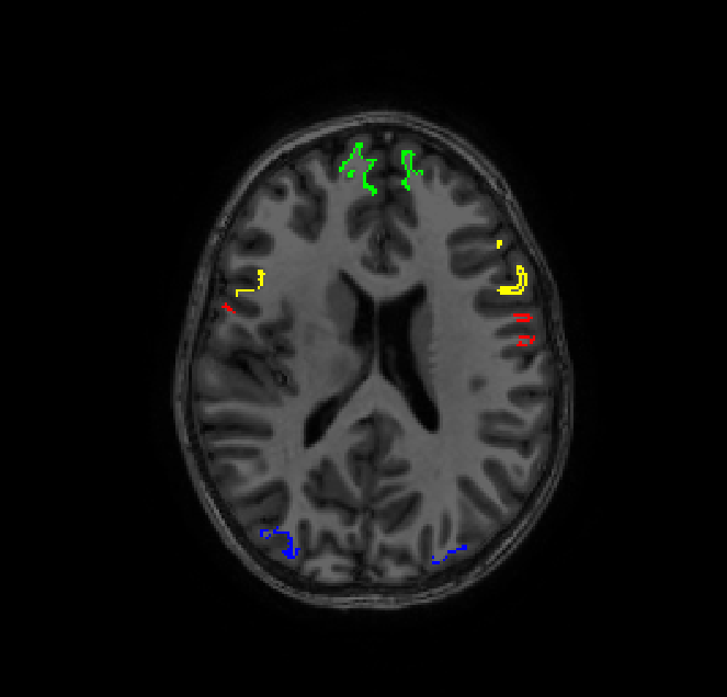
I empirically determined this ordering of labels in this notebook but I removed BA*, cortex, entorhinal, MT and V* labels since they overlap with the 2009 atlas. seeds.txt now contains 148 (74 labels * 2 hemispheres) paths to our volumes of interest.

Just for a sanity check, let’s overlay a few of these volumes on the T1 image in Freesurfer space:

Now we’re ready to being tractography (If you’re still with me, I applaud you)

Tractography

At this point, you’re going to need a big computer. Each of these 148 seed regions can run independently, so if you have access to a compute cluster, by all means use it. For each probtracking run, we’re going to do this:

$ probtrackx2 -x label/lh.G_and_S_cingul-Ant.nii.gz \
    -s bedpostx/merged \
    -m bedpostx/nodif_brain_mask \
    -l \
    --usef \
    --s2tastext \
    --os2t \
    --onewaycondition \
    -c 0.2 \
    -S 2000 \
    --steplength=0.5 \
    -P 5000 \
    --fibthresh=0.01 \
    --distthresh=0.0 \
    --sampvox=0.0 \
    --xfm=bedpostx/xfms/fs2fa.mat \
    --avoid=anat/ventricles.nii.gz \
    --seedref=anat/fs.nii.gz \
    --forcedir \
    --opd \
    -V 1 \
    --omatrix1 \
    --dir=results/lh.G_and_S_cingul-Ant.nii.gz.probtrackx2/ \
    --waypoints=waypoints.txt \
    --waycond='OR' \
    --targetmasks=seeds.txt

It’s an exercise to the reader to generate 148 of these scripts. I suggest python :)

Let’s walk through the options because I’ve wasted many months of compute time generating crap results.

• -x is the seed. This will differ for each run.
• -s is the merged samples from bedpostx.
• -m is the non-diffusion brain mask.
• -l performs loop checks on paths.
• -usef uses FA for constrain prob tracking.
• --s2tastext outputs text files for all generated tracts. You must set this along with -os2t to generate the proper output files.
• --os2t Outputs seeds to target images. One per voxel in the seed. There can be quite a lot of these files.
• --onewaycondition applies waypoint conditions to each half of the tract separately (see --waypoints).
• -c 0.2 constrains curvature of the generated tracts. This is the default.
• -S 2000 Each tract is created by at the most 2000 steps.
• --steplength=0.5 gives step length in mm. -S * –steplength` is the maximum length a tract can be.
• -P 5000 the number of sample tracts generated. This number above all else determines the time it takes to run this.
• --fibthresh=0.01 thresholds the point at which probtrack will consider orientations of differing directions.
• --distthresh=0.0 samples shorter than this length are discarded.
• --sampvox=0.0 randomly sample the points with 0.0 mm sphere of the seed voxel. I set this to zero because I trust the incoming seed.
• --xfm=bedpostx/xfms/fs2fa.mat this sets the linear transform from seed space to DTI space.
• --meshspace=freesurfer We’re using Freesurfer meshes.
• --avoid=$ventricles Generated samples to run into the --avoid image (or iamges) are flat-out rejected. Anatomically speaking, fiber tracts do not pass through the ventricles.
• --seedref=anat/brain.nii.gz this merely gives the reference space for the seeds. Output images are of this size and shape.
• --forcedir use the results directory given, don’t create a new one.
• --opd output the distributions of the samples.
• -V 1 Verbosity level
• --omatrix1 We’re interested in the seed-to-targets matrix.
• --dir=results/lh.G_and_S_cingul-Ant.gii.probtrackx2/ directory for results.
• --waypoints=waypoints.txt this file, which for me contains the paths to the white matter binarized images, requires that generated samples pass through these way points. Samples that don’t are rejected. I’m assuming that pathways I care about pass through white matter.
• --waycond='OR' this determines the boolean logic for rejecting (or keeping) pathways given by --waypoints. In this instance, I only want the stream lines to pass through the left or right white matter, not necessarily both.
• --targetmasks=seeds.txt This file gives path names to the seeds of interest. As I said before, this is every region from the brain.

The time it takes probtrackx2 to finish a region depends on the size of the region. As you can see above in the cortical parcellation picture, not all regions are the same size. Hence some runs don’t take very long (~90 minutes) and others will take a very long time, upwards of 96 hours on modern hardware. Having done this processing on a few subjects, I can say that all told these runs take about 30 days of compute time per subject. Grab a coffee and pillow.

Analysis

When everything is finished, we’d like to visualize the NxN connectivity matrix. We get two important outputs from our probtrackx2 runs. fdt_paths.nii.gz can be overlayed on the reference file and contains a count at every voxel of how many streamlines passed through that voxel. The other output of interest is matrix_seeds_to_all_targets.nii.gz. This is a 2D voxel-by-target matrix. By collapsing across all seed voxels and dividing by the total number of streamlines generated during the run, we generate a 1xN array of percentages representing the proportion of streamlines that reached each target. By doing this for all 148 output matrices and stacking the arrays, we generate a 148x148 connectivity matrix.

Here is my implementation in python:

import numpy as np
import matplotlib as mpl
plt = mpl.pyplot
import nibabel
import os

def collapse_probtrack_results(waytotal_file, matrix_file):
    with open(waytotal_file) as f:
        waytotal = int(f.read())
    data = nibabel.load(matrix_file).get_data()
    collapsed = data.sum(axis=0) / waytotal * 100.
    return collapsed

matrix_template = 'results/{roi}.nii.gz.probtrackx2/matrix_seeds_to_all_targets.nii.gz'
processed_seed_list = [s.replace('.nii.gz','').replace('label/', '')
    for s in open('seeds.txt').read().split('\n')
    if s]
N = len(processed_seed_list)
conn = np.zeros((N, N))
rois=[]
idx = 0
for roi in processed_seed_list:
    matrix_file = template.format(roi=roi)
    seed_directory = os.path.dirname(result)
    roi = os.path.basename(seed_directory).replace('.nii.gz.probtrackx2', '')
    waytotal_file = os.path.join(seed_directory, 'waytotal')
    rois.append(roi)
    try:
        # if this particular seed hasn't finished processing, you can still
        # build the matrix by catching OSErrors that pop up from trying
        # to open the non-existent files
        conn[idx, :] = collapse_probtrack_results(waytotal_file, matrix_file)
    except OSError:
        pass
    idx += 1

# figure plotting
fig = plt.figure()
ax = fig.add_subplot(111)
cax = ax.matshow(conn, interpolation='nearest', )
cax.set_cmap('hot')
caxes = cax.get_axes()

# set number of ticks
caxes.set_xticks(range(len(new_order)))
caxes.set_yticks(range(len(new_order)))

# label the ticks
caxes.set_xticklabels(new_order, rotation=90)
caxes.set_yticklabels(new_order, rotation=0)

# axes labels
caxes.set_xlabel('Target ROI', fontsize=20)
caxes.set_ylabel('Seed ROI', fontsize=20)

# Colorbar
cbar = fig.colorbar(cax)
cbar.set_label('% of streamlines from seed to target', rotation=-90, fontsize=20)

# title text
title_text = ax.set_title('Structural Connectivity with Freesurfer Labels & ProbtrackX2',
    fontsize=26)
title_text.set_position((.5, 1.10))

Link to full image

The diagonal is connectivity from the seed to itself so it makes sense that is very “hot”. Close to off-diagonal we see the most connectivity which also makes sense because I’ve constrained the list to be anatomically “nearby”. I’ve got a few ideas about what to do with this matrices, but I’ll save that for another day.